Excel help

[RU_]

Hi all, hoping you might be able to help me with something that will streamline some of my employment excel work.

I’ve got two excel spreadsheets.
Spreadsheet A is from last week and outdated.
Spreadsheet B is from this week and the current one with my updated project list.

Spreadsheet A has my notes in column M of excel but doesn’t have my latest projects list.

Can I merge the job numbers in Column A and the notes of Column M in Spreadsheet A (outdated spreadsheet with notes) into spreadsheet B so that the vacant notes rows will be my new projects?

 

[Cleavy]

tried a vlookup?

 

[RU_]

tried a vlookup?

I’ve tried and it won’t work, not sure what I’m doing wrong

 

[kaiserchief13]

Xlookup? index/match? vba macro using row.count to get row number variable?

Maybe provide screenshots as it's not 100% clear what the problem is

 

[randyzany]

Seems the OP query has been answered so I hope the OP doesn't mind using this thread instead of making a new one.

I want to create a table or spreadsheet (whichever is easier) from 2 sets of data which are small tables themselves.

1 set of data contains the column reference of a particular value and the other set of data contains the row reference of that value.

The Column Headers are the generic C1, C2, C3, etc.. and the Row Headers R1, R2, R3, etc...



I have these sets of data in the form of 2 mini tables:

VALUE: 1, 2, etc..
COLUMN: 8, 12, etc..


VALUE: 1, 2, etc..
ROW: 5, 6, etc..

From these mini tables I want to make a larger table that places Value 1 in Column 8 and Row 5, Value 2 in C12,R6, etc..

Been googling for a while with no luck in finding out to combine data from 2 tables to form a new one.

 

[Caesar]

Seems the OP query has been answered so I hope the OP doesn't mind using this thread instead of making a new one.

I want to create a table or spreadsheet (whichever is easier) from 2 sets of data which are small tables themselves.

1 set of data contains the column reference of a particular value and the other set of data contains the row reference of that value.

The Column Headers are the generic C1, C2, C3, etc.. and the Row Headers R1, R2, R3, etc...



I have these sets of data in the form of 2 mini tables:

VALUE: 1, 2, etc..
COLUMN: 8, 12, etc..


VALUE: 1, 2, etc..
ROW: 5, 6, etc..

From these mini tables I want to make a larger table that places Value 1 in Column 8 and Row 5, Value 2 in C12,R6, etc..

Been googling for a while with no luck in finding out to combine data from 2 tables to form a new one.

the search phrases I would use for this problem are 'join tables in Excel' and 'convert table to matrix in Excel'

there are a few different ways to do it, but (assuming you don't have duplicate values) I would use Power Query to join the two tables on the Value column, then use the Pivot Column function to create your columns (under advanced options, select Don't Aggregate)

example file attached

 

[randyzany]

When I first started searching for a solution for this task on Excel I just assumed that it would be fairly straightforward and need only the Excel basics (like stuff you learnt for school assignments) for it to complete it. Have to brush up on those matrices and arrays, thanks for the hints.

Oh and I appreciate the template you've uploaded, thanks again.

 

[CrowToon]

If I have 2 drop down boxes can I set up a formula so that depending on what value is selected from the drop down boxes (worded selections) it then displays a result in a third box.

For example, the first drop down box are tasks and the second drop down box are departments. Can I then, depending on what someone selects, then display, for example, someone's name?

Also is an excel spreadsheet the best way to achieve this or is there something better?

I got as far as dependent drop down boxes via tutorials but I can't find a way to marry it all up.

 

[Engimal v3]

If I have 2 drop down boxes can I set up a formula so that depending on what value is selected from the drop down boxes (worded selections) it then displays a result in a third box.

For example, the first drop down box are tasks and the second drop down box are departments. Can I then, depending on what someone selects, then display, for example, someone's name?

Also is an excel spreadsheet the best way to achieve this or is there something better?

I got as far as dependent drop down boxes via tutorials but I can't find a way to marry it all up.

As far as if Excel is the best tool for it, you haven't given enough detail on what you're trying to achieve.

What you're describing there is pretty simple though. Easiest way in my mind would be to put Data Validation on the first two cells and set it to a list of allowed values that you set elsewhere on the sheet (or another sheet). In the third cell, you apply a formula to concatenate the values from the first two cells, and then do a VLookup to another sheet where you're storing Key/Value pairs.

That way you don't have to muck around with VBA or any ActiveX stuff.

 

[smauge]

I always find tips here: https://www.youtube.com/@LeilaGharani. The youtube channel is pretty helpful. Check it out.

If you find this process challenging, you might also consider learning how to develop from scratch your own Excel macros or small applications to automate such tasks. This can be incredibly useful and save you a lot of time in the long run.

 

[X_box_X]

I'm hoping someone can help with what I'm hoping is an easy fix.






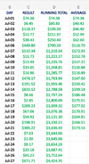
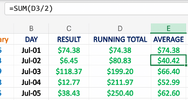
Column 'E' is simply Column D / QUANTITY. I achieve this by manually typing =SUM(D2/1), =SUM(D3/2) etc etc.
I.e.








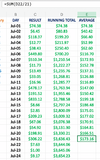
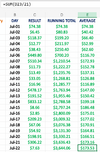
The issue is, when I drag down to the next cell in column E (I.e. drag cell E22 to cell E23 in the above example), it doesn't do the calculation I need. I have to enter it manually.

This is what I mean...




The equation automatically reverts to =SUM(D23/21) when I need it to automatically revert to =SUM(D23/22). Unless I manually adjust the figure, the equation will remain as a divisible of 21. I.e. D24/21, D25/21 etc etc.

How do I code this so the amount divisible automatically increases by one as I drag the previous cell into the next row?

 

[kaiserchief13]

I'm hoping someone can help with what I'm hoping is an easy fix.



View attachment 2112371


Column 'E' is simply Column D / QUANTITY. I achieve this by manually typing =SUM(D2/1), =SUM(D3/2) etc etc.
I.e.

View attachment 2112370


View attachment 2112375

View attachment 2112378

The issue is, when I drag down to the next cell in column E (I.e. drag cell E22 to cell E23 in the above example), it doesn't do the calculation I need. I have to enter it manually.

This is what I mean...

View attachment 2112382


The equation automatically reverts to =SUM(D23/21) when I need it to automatically revert to =SUM(D23/22). Unless I manually adjust the figure, the equation will remain as a divisible of 21. I.e. D24/21, D25/21 etc etc.

How do I code this so the amount divisible automatically increases by one as I drag the previous cell into the next row?

E2=C2/(COUNTA($B$2:B2)). Drag formula down

 

[X_box_X]

E2=C2/(COUNTA($B$2:B2)). Drag formula down

Thanks for replying

What am I doing wrong here?

 

[kaiserchief13]

Thanks for replying

What am I doing wrong here?

View attachment 2112405

Remove the 'e2

 

[X_box_X]

Remove the 'e2

Amazing!!!

Thanks mate.

It was the D column I needed to do my calculation, but everything else was spot on!

 

[burge13]

I'm hoping someone can help with what I'm hoping is an easy fix.



View attachment 2112371


Column 'E' is simply Column D / QUANTITY. I achieve this by manually typing =SUM(D2/1), =SUM(D3/2) etc etc.
I.e.

View attachment 2112370


View attachment 2112375

View attachment 2112378

The issue is, when I drag down to the next cell in column E (I.e. drag cell E22 to cell E23 in the above example), it doesn't do the calculation I need. I have to enter it manually.

This is what I mean...

View attachment 2112382


The equation automatically reverts to =SUM(D23/21) when I need it to automatically revert to =SUM(D23/22). Unless I manually adjust the figure, the equation will remain as a divisible of 21. I.e. D24/21, D25/21 etc etc.

How do I code this so the amount divisible automatically increases by one as I drag the previous cell into the next row?

Good results, what were you punting for this